Isophotal measurements

Position and shape

The following quantities are derived from the spatial distribution \(\cal S\) of pixels detected above the detection threshold (see description).

Important

Unless otherwise noted, the pixel values used for computing "isophotal" positions and shapes are taken from the filtered, background-subtracted detection image.

Note

Unless otherwise noted, all parameter names given below are only prefixes. They must be followed by _IMAGE if the results shall be expressed in pixel coordinates or _WORLD, _SKY, _J2000 or _B1950 for WCS coordinates (see Positions and shapes).

Limits: XMIN, YMIN, XMAX, YMAX

These coordinates define two corners of a rectangle which encloses the detected object:

\begin{eqnarray} {\tt XMIN} & = & \min_{i \in {\cal S}} x_i,\\ {\tt YMIN} & = & \min_{i \in {\cal S}} y_i,\\ {\tt XMAX} & = & \max_{i \in {\cal S}} x_i,\\ {\tt YMAX} & = & \max_{i \in {\cal S}} y_i, \end{eqnarray}

where \(x_i\) and \(y_i\) are respectively the x-coordinate and y-coordinate of pixel \(i\).

Barycenter: X, Y

Barycenter coordinates generally define the position of the “center” of a source, although this definition can be inadequate or inaccurate if its spatial profile shows a strong skewness or very large wings. X and Y are simply computed as the first order moments of the profile:

\begin{eqnarray} {\tt X} & = & \overline{x} = \frac{\displaystyle \sum_{i \in {\cal S}} p^{(f)}_i x_i}{\displaystyle \sum_{i \in {\cal S}} p^{(f)}_i},\\ {\tt Y} & = & \overline{y} = \frac{\displaystyle \sum_{i \in {\cal S}} p^{(f)}_i y_i}{\displaystyle \sum_{i \in {\cal S}} p^{(f)}_i}, \end{eqnarray}

where \(p^{(f)}_i\) is the value of the pixel \(i\) in the (filtered) detection image. In practice, \(x_i\) and \(y_i\) are summed relative to XMIN and YMIN in order to reduce roundoff errors in the summing.

Position of the peak: XPEAK, YPEAK

It is sometimes useful to have the position XPEAK, YPEAK of the pixel with maximum intensity in a detected object, for instance when working with likelihood maps, or when searching for artifacts. For better robustness, PEAK coordinates are computed on filtered profiles if available. On symmetrical profiles, PEAK positions and barycenters coincide within a fraction of pixel (XPEAK and YPEAK coordinates are quantized by steps of 1 pixel, hence XPEAK_IMAGE and YPEAK_IMAGE are integers). This is no longer true for skewed profiles, therefore a simple comparison between PEAK and barycenter coordinates can be used to identify asymmetrical objects on well-sampled images.

Second-order moments: X2, Y2, XY

(Centered) second-order moments are convenient for measuring the spatial spread of a source profile. In SExtractor they are computed with:

\begin{eqnarray} {\tt X2} & = \overline{x^2} = & \frac{\displaystyle \sum_{i \in {\cal S}} p^{(f)}_i x_i^2}{\displaystyle \sum_{i \in {\cal S}} p^{(f)}_i} - \overline{x}^2,\\ {\tt Y2} & = \overline{y^2} = & \frac{\displaystyle \sum_{i \in {\cal S}} p^{(f)}_i y_i^2}{\displaystyle \sum_{i \in {\cal S}} p^{(f)}_i} - \overline{y}^2,\\ {\tt XY} & = \overline{xy} = & \frac{\displaystyle \sum_{i \in {\cal S}} p^{(f)}_i x_i y_i}{\displaystyle \sum_{i \in {\cal S}} p^{(f)}_i} - \overline{x}\,\overline{y}, \end{eqnarray}

These expressions are more subject to roundoff errors than if the 1st-order moments were subtracted before summing, but allow both 1st and 2nd order moments to be computed in one pass. Roundoff errors are however kept to a negligible value by measuring all positions relative here again to XMIN and YMIN.

Basic shape parameters: A, B, THETA

These parameters are intended to describe the detected object as an elliptical shape. A and B are the lengths of the semi-major and semi-minor axes, respectively. More precisely, they represent the maximum and minimum spatial dispersion of the object profile along any direction. THETA is the position-angle of the A axis relative to the first image axis. It is counted positive in the direction of the second axis.

Here is how shape parameters are computed. 2nd-order moments can easily be expressed in a referential rotated from the \(x,y\) image coordinate system by an angle +\(\theta\):

(9)\[\begin{split} \begin{array}{lcrrr} \overline{x_{\theta}^2} & = & \cos^2\theta\:\overline{x^2} & +\,\sin^2\theta\:\overline{y^2} & -\,2 \cos\theta \sin\theta\:\overline{xy},\\ \overline{y_{\theta}^2} & = & \sin^2\theta\:\overline{x^2} & +\,\cos^2\theta\:\overline{y^2} & +\,2 \cos\theta \sin\theta\:\overline{xy},\\ \overline{xy_{\theta}} & = & \cos\theta \sin\theta\:\overline{x^2} & -\,\cos\theta \sin\theta\:\overline{y^2} & +\,(\cos^2\theta - \sin^2\theta)\:\overline{xy}. \end{array}\end{split}\]

One can find the angle(s) \(\theta_0\) for which the variance is minimized (or maximized) along \(x_{\theta}\):

(10)\[{\left.\frac{\partial \overline{x_{\theta}^2}}{\partial \theta} \right|}_{\theta_0} = 0,\]

which leads to

(11)\[ 2 \cos\theta \sin\theta_0\:(\overline{y^2} - \overline{x^2}) + 2 (\cos^2\theta_0 - \sin^2\theta_0)\:\overline{xy} = 0.\]

If \(\overline{y^2} \neq \overline{x^2}\), this implies:

(12)\[\tan 2\theta_0 = 2 \frac{\overline{xy}}{\overline{x^2} - \overline{y^2}},\]

a result which can also be obtained by requiring the covariance \(\overline{xy_{\theta_0}}\) to be null. Over the domain \([-\pi/2, +\pi/2[\), two different angles — with opposite signs — satisfy (12). By definition, THETA is the position angle for which \(\overline{x_{\theta}^2}\) is maximized. THETA is therefore the solution to (12) that has the same sign as the covariance \(\overline{xy}\). A and B can now simply be expressed as:

\begin{eqnarray} {\tt A}^2 & = & \overline{x^2}_{\tt THETA},\ \ \ {\rm and}\\ {\tt B}^2 & = & \overline{y^2}_{\tt THETA}. \end{eqnarray}

A and B can be computed directly from the 2nd-order moments, using the following equations derived from (9) after some algebra:

\begin{eqnarray} {\tt A}^2 & = & \frac{\overline{x^2}+\overline{y^2}}{2} + \sqrt{\left(\frac{\overline{x^2}-\overline{y^2}}{2}\right)^2 + \overline{xy}^2},\\ {\tt B}^2 & = & \frac{\overline{x^2}+\overline{y^2}}{2}, - \sqrt{\left(\frac{\overline{x^2}-\overline{y^2}}{2}\right)^2 + \overline{xy}^2}. \end{eqnarray}

Note that A and B are exactly halves the \(a\) and \(b\) parameters computed by the COSMOS image analyser [17]. Actually, \(a\) and \(b\) are defined in [17] as the semi-major and semi-minor axes of an elliptical shape with constant surface brightness, which would have the same 2nd-order moments as the analyzed object.

By-products of shape parameters: ELONGATION and ELLIPTICITY

These parameters [1] are directly derived from A and B:

\begin{eqnarray} {\tt ELONGATION} & = & \frac{\tt A}{\tt B}\ \ \ \ \ \mbox{and}\\ {\tt ELLIPTICITY} & = & 1 - \frac{\tt B}{\tt A}. \end{eqnarray}

[1]

These parameters are dimensionless, and for historical reasons do not accept suffixes such as _IMAGE or _WORLD.

Ellipse parameters: CXX, CYY, CXY

A, B and THETA are not very convenient to use when, for instance, one wants to know if a particular SExtractor detection extends over some position. For this kind of application, three other ellipse parameters are provided; CXX, CYY, and CXY. They do nothing more than describing the same ellipse, but in a different way: the elliptical shape associated to a detection is now parameterized as

(16)\[ {\tt CXX} (x-\overline{x})^2 + {\tt CYY} (y-\overline{y})^2 + {\tt CXY} (x-\overline{x})(y-\overline{y}) = R^2,\]

where \(R\) is a parameter which scales the ellipse, in units of A (or B). Generally, the isophotal limit of a detected object is well represented by \(R\approx 3\) (Fig. 3). Ellipse parameters can be derived from the 2nd order moments:

\begin{eqnarray} {\tt CXX} & = & \frac{\cos^2 {\tt THETA}}{{\tt A}^2} + \frac{\sin^2 {\tt THETA}}{{\tt B}^2} = \frac{\overline{y^2}}{\overline{x^2} \overline{y^2} - \overline{xy}^2}\\ {\tt CYY} & = & \frac{\sin^2 {\tt THETA}}{{\tt A}^2} + \frac{\cos^2 {\tt THETA}}{{\tt B}^2} = \frac{\overline{x^2}}{\overline{x^2} \overline{y^2} - \overline{xy}^2}\\ {\tt CXY} & = & 2 \,\cos {\tt THETA}\,\sin {\tt THETA} \left( \frac{1}{{\tt A}^2} - \frac{1}{{\tt B}^2}\right) = -2\, \frac{\overline{xy}}{\overline{x^2} \overline{y^2} - \overline{xy}^2}. \end{eqnarray}

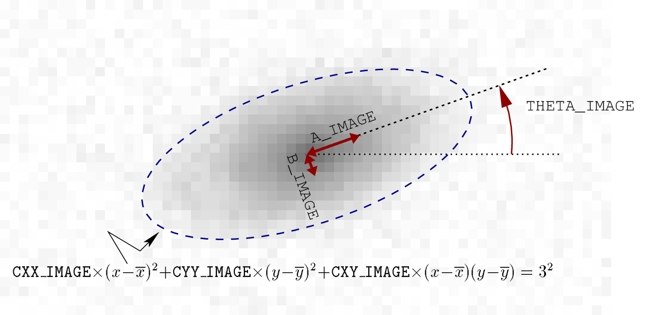
Fig. 3 Meaning of basic shape parameters.

Position uncertainties: ERRX2, ERRY2, ERRXY, ERRA, ERRB, ERRTHETA, ERRCXX, ERRCYY, ERRCXY

Uncertainties on the position of the barycenter can be estimated using photon statistics. In practice, such estimates are a lower-value of the full uncertainties because they do not include, for instance, the contribution of detection biases or contamination by neighbors. Furthermore, SExtractor does not currently take into account possible correlations of the noise between adjacent pixels. Hence variances simply write:

\begin{eqnarray} {\tt ERRX2} & = {\rm var}(\overline{x}) = & \frac{\displaystyle \sum_{i \in {\cal S}} \sigma^2_i (x_i-\overline{x})^2} {\displaystyle \left(\sum_{i \in {\cal S}} p^{(f)}_i\right)^2},\\ {\tt ERRY2} & = {\rm var}(\overline{y}) = & \frac{\displaystyle \sum_{i \in {\cal S}} \sigma^2_i (y_i-\overline{y})^2} {\displaystyle \left(\sum_{i \in {\cal S}} p^{(f)}_i\right)^2},\\ {\tt ERRXY} & = {\rm cov}(\overline{x},\overline{y}) = & \frac{\displaystyle \sum_{i \in {\cal S}} \sigma^2_i (x_i-\overline{x})(y_i-\overline{y})} {\displaystyle \left(\sum_{i \in {\cal S}} p^{(f)}_i\right)^2}. \end{eqnarray}

\(\sigma_i\) is the flux uncertainty estimated for pixel \(i\):

\[\sigma^2_i = {\sigma_B}^2_i + \frac{p^{(f)}_i}{g_i},\]

where \({\sigma_B}_i\) is the local background noise and \(g_i\) the local gain — conversion factor — for pixel \(i\) (see Effect of weighting for more details). Semi-major axis ERRA, semi-minor axis ERRB, and position angle ERRTHETA of the \(1\sigma\) position error ellipse are computed from the covariance matrix exactly like for basic shape parameters:

\begin{eqnarray} {\tt ERRA}^2 & = & \frac{{\rm var}(\overline{x})+{\rm var}(\overline{y})}{2} + \sqrt{\left(\frac{{\rm var}(\overline{x})-{\rm var}(\overline{y})}{2}\right)^2 + {\rm cov}^2(\overline{x},\overline{y})},\\ {\tt ERRB}^2 & = & \frac{{\rm var}(\overline{x})+{\rm var}(\overline{y})}{2} - \sqrt{\left(\frac{{\rm var}(\overline{x})-{\rm var}(\overline{y})}{2}\right)^2 + {\rm cov}^2(\overline{x},\overline{y})},\\ \tan (2{\tt ERRTHETA}) & = & 2 \,\frac{{\rm cov}(\overline{x},\overline{y})} {{\rm var}(\overline{x}) - {\rm var}(\overline{y})}. \end{eqnarray}

And the error ellipse parameters are:

\begin{eqnarray} {\tt ERRCXX} & = & \frac{\cos^2 {\tt ERRTHETA}}{{\tt ERRA}^2} + \frac{\sin^2 {\tt ERRTHETA}}{{\tt ERRB}^2} = \frac{{\rm var}(\overline{y})}{{\rm var}(\overline{x}) {\rm var}(\overline{y}) - {\rm cov}^2(\overline{x},\overline{y})},\\ {\tt ERRCYY} & = & \frac{\sin^2 {\tt ERRTHETA}}{{\tt ERRA}^2} + \frac{\cos^2 {\tt ERRTHETA}}{{\tt ERRB}^2} = \frac{{\rm var}(\overline{x})}{{\rm var}(\overline{x}) {\rm var}(\overline{y}) - {\rm cov}^2(\overline{x},\overline{y})},\\ {\tt ERRCXY} & = & 2 \cos {\tt ERRTHETA}\sin {\tt ERRTHETA} \left( \frac{1}{{\tt ERRA}^2} - \frac{1}{{\tt ERRB}^2}\right)\\ & = & -2 \frac{{\rm cov}(\overline{x},\overline{y})}{{\rm var}(\overline{x}) {\rm var}(\overline{y}) - {\rm cov}^2(\overline{x},\overline{y})}. \end{eqnarray}

Handling of “infinitely thin” detections

Apart from the mathematical singularities that can be found in some of the above equations describing shape parameters (and which SExtractor is able to handle, of course), some detections with very specific shapes may yield unphysical parameters, namely null values for B, ERRB, or even A and ERRA. Such detections include single-pixel objects and horizontal, vertical or diagonal lines which are 1-pixel wide. They will generally originate from glitches; but strongly undersampled and/or low S/N genuine sources may also produce such shapes.

For basic shape parameters, the following convention was adopted: if the light distribution of the object falls on one single pixel, or lies on a sufficiently thin line of pixels, which we translate mathematically by

(21)\[ \overline{x^2}\,\overline{y^2} - \overline{xy}^2 < \rho^2,\]

then \(\overline{x^2}\) and \(\overline{y^2}\) are incremented by \(\rho\). SExtractor sets \(\rho=1/12\), which is the variance of a 1-dimensional top-hat distribution with unit width. Therefore \(1/\sqrt{12}\) represents the typical minor-axis values assigned (in pixels units) to undersampled sources in SExtractor.

Positional errors are more difficult to handle, as objects with very high signal-to-noise can yield extremely small position uncertainties, just like singular profiles do. Therefore SExtractor first checks that (21) is true. If this is the case, a new test is conducted:

(22)\[ {\rm var}(\overline{x})\,{\rm var}(\overline{y}) - {\rm covar}^2(\overline{x}, \overline{y}) < \rho^2_e,\]

where \(\rho_e\) is arbitrarily set to \(\left( \sum_{i \in {\cal S}} \sigma^2_i \right) / \left(\sum_{i \in {\cal S}} p_i\right)^2\). If (22) is true, then \(\overline{x^2}\) and \(\overline{y^2}\) are incremented by \(\rho_e\).

Isophotal areas: ISOAREA, ISOAREAF

An isophotal area is defined as the number of pixels with values exceeding some threshold above the background. Isophotal areas played an important role in the 80's and the 90's by providing, at a small computing cost, morphometric quantities complementary to second-order moments. SExtractor computes two isophotal areas inside the detection footprint:

• ISOAREAF applies to the (filtered) detection image, above the detection threshold.

• ISOAREA applies to the measurement image, with the additional constraint that the background-subtracted value of measurement image pixels must exceed the threshold set with the ANALYSIS_THRESH configuration parameter.

Photometry

Important

Unless otherwise noted, the pixel values used for computing "isophotal" fluxes and surface brightnesses are taken from the background-subtracted measurement image.

Isophotal flux: FLUX_ISO

FLUX_ISO is computed simply by integrating the background-subracted pixels values \(p_i\) from the measurement image within the detection footprint

(23)\[ {\tt FLUX\_ISO} = F_{\rm iso} = \sum_{i \in {\cal S}} p_i.\]

SExtractor also provides an estimation of the uncertainty FLUXERR_ISO, a magnitude MAG_ISO and a magnitude error estimate MAGERR_ISO: see Fluxes and magnitudes.

Corrected isophotal magnitude: MAG_ISOCOR

Note

Corrected isophotal magnitudes are now deprecated; they remain in SExtractor v2.x for compatibility with SExtractor v1.

MAG_ISOCOR magnitudes are a quick-and-dirty way of retrieving the fraction of flux lost by isophotal magnitudes.

If one makes the assumption that the intensity profiles of faint objects recorded in the frame are roughly Gaussian because of atmospheric blurring, then the fraction \(\eta = \frac{F_{\rm iso}}{F_{\rm tot}}\) of the total flux enclosed within a particular isophote reads [18]:

(24)\[ \left(1-\frac{1}{\eta}\right ) \ln (1-\eta) = \frac{A\,t}{F_{\rm iso}},\]

where \(A\) is the area and \(t\) the threshold related to this isophote. :eq:isocor is not analytically invertible, but a good approximation to \(\eta\) (error \(< 10^{-2}\) for \(\eta > 0.4\)) can be done with the second-order polynomial fit:

(25)\[ \eta \approx 1 - 0.1961 \frac{A\,t}{F_{\rm iso}} - 0.7512 \left( \frac{A\,t}{F_{\rm iso}}\right)^2.\]

A “total” magnitude MAG_ISOCOR estimate is then

(26)\[ {\tt MAG\_ISOCOR} = {\tt MAG\_ISO} + 2.5 \log_{10} \eta.\]

Clearly the MAG_ISOCOR correction works best with stars; and although it gives reasonably accurate results with most disk galaxies, it breaks down for ellipticals because of the broader wings in the profiles.

Peak value: FLUX_MAX

FLUX_MAX is the peak pixel value (above the local background) in the measurement image. Note that it may not correspond to the pixel with coordinates given by XPEAK and YPEAK (see Position of the peak) if FILTER is set to Y or if the measurement image differs from the detection image.

CLASS_STAR classifier

Note

The CLASS_STAR classifier has been superseded by the SPREAD_MODEL estimator (see Model-based star-galaxy separation: SPREAD_MODEL), which offers better performance by making explicit use of the full, variable PSF model.

A good discrimination between stars and galaxies is essential for both galactic and extragalactic statistical studies. The common assumption is that galaxy images look more extended or fuzzier than those of stars (or QSOs). SExtractor provides the CLASS_STAR catalog parameter for separating both types of sources. The CLASS_STAR classifier relies on a multilayer feed-forward neural network trained using supervised learning to estimate the a posteriori probability [19, 20] of a SExtractor detection to be a point source or an extended object. Below is a shortened description of the estimator, see [12] for more details.

Inputs and outputs

The neural network is a multilayer Perceptron with a single fully connected, hidden layers. Of all neural networks it is probably the best-studied, and it has been intensively applied with success for many classification tasks.

The classifier (Fig. 4) has 10 inputs:

• 8 isophotal areas \(A_0..A_7\), measured at isophotes exponentially spaced between the analysis threshold (which may be modified with the ANALYSIS_THRESH configuration parameter) and the object's peak pixel value

• The object's peak pixel value above the local background \(I_{\mathrm max}\)

• A seeing input, which acts as a tuning button.

The output layer contains only one neuron, as "star" and "galaxy" are two classes mutually exclusive. The output value is a "stellarity index", which for images that reasonably match those of the training sample is an estimation of the a posteriori probability for the classified object to be a point-source. Hence a CLASS_STAR close to 0 means that the object is very likely a galaxy, and 1 that it is a star. In practice, real data always differ at least slightly from the training sample, and the CLASS_STAR output is often a poor approximation of the expected a posteriori probabilities. Nevertheless, a CLASS_STAR value closer to 0 or 1 normally indicates a higher confidence in the classification, and the balance between sample completeness and purity may still be adjusted by tweaking the decision threshold .

Fig. 4 Architecture of SExtractor's CLASS_STAR classifier

The seeing input must be set by the user with the SEEING_FWHM configuration parameter. If SEEING_FWHM is set to 0, it is automatically measured on the PSF model which must be provided (using the PSF_NAME configuration parameter).

If no PSF model is available, the SEEING_FWHM configuration parameter must be adjusted by the user to match the actual average PSF FWHM on the image. The accuracy with which SEEING_FWHM must be set for optimal results ranges from \(\pm 20\%\) for bright sources to about \(\pm 5\%\) for the faintest (Fig. 5). SEEING_FWHM is expressed in arcseconds. The PIXEL_SCALE configuration parameter must therefore also be set by the user if WCS information is missing from the FITS image header. There are several ways to measure, directly or indirectly, the size of point sources in SExtractor; they may lead to slightly discordant results, depending on the exact shape of the PSF. The measurement FWHM_IMAGE (although not the most reliable as an image quality estimator) sets the reference when it comes to setting SEEING_FWHM.

One may check that the SEEING_FWHM is set correctly by making sure that the typical CLASS_STAR value of unclassifiable sources at the faint end of the catalog hovers around the 0.5 mark.

Fig. 5 Architecture of SExtractor's CLASS_STAR classifier

Training

This section gives some insight on how the CLASS_STAR classifier has been trained. The main issue with supervised machine learning is the labeling of the large training sample. Hopefully a big percentage of contemporary astronomical images share a common set of generic features, which can be simulated with sufficient realism to create a large training sample together with the ground truth (labels). The CLASS_STAR classifier was trained on such a sample of artificial images.

Six hundred \(512\times512\) simulation images containing stars and galaxies were generated to train the network using an early prototype of the SkyMaker package [21]. They were done in the blue band, where galaxies present very diversified aspects. The two parameters governing the shape of the PSF (seeing FWHM and Moffat \(\beta\) parameter [22]) were chosen randomly with \(0.025\le\) FWHM \(\le 5.5\) and \(2\le\beta\le4\). Note that the Moffat function used in the simulation is a poor approximation to diffraction-limited images, hence the CLASS_STAR classifier is not optimized for space-based images. The pixel scale was always taken less than \(\approx 0.7\) FWHM to warrant correct sampling of the image. Bright galaxies are simply too rare in the sky to constitute a significant training sample on such a small number of simulations. So, keeping a constant comoving number density, we increased artificially the number of nearby galaxies by making the volume element proportional to \(zdz\). Stars were given a number-magnitude distribution identical to that of galaxies. Therefore any pattern presented to the network had a 50% chance to correspond to a star or a galaxy, irrespective of magnitude [2]. Crowding in the simulated images was higher than what one sees on real images of high galactic latitude fields, allowing for the presence of many “difficult cases” (close double stars, truncated profiles, etc...) that the neural network classifier had to deal with.

SExtractor was run on each image with 8 different extraction thresholds. This led to a catalog with about \(10^6\) entries with the 10 input parameters plus the class label. Back-propagation learning took about 15 min on a SUN SPARC20 workstation. The final set of synaptic weights was saved to the file default.nnw , ready to be used in “feed-forward” mode during source extraction.

[2]

Faint galaxies have less chance being detected than faint stars, but it has little effect because the ones that are lost at a given magnitude are predominantly the most extended and consequently the easiest to classify.